MS-Ana
Maintained by ppernot
analysis.R script
For each DMS-MS/MS experiment as given in a series in the taskTable
file, the series of metabolites given in tgTable is analyzed. The aim
of the analysis is to integrate the peak (i.e., to estimate the area)
corresponding to each metabolite.
Peak model
In the present version, a Gaussian peak shape is used. The formula of a
Gaussian function is
where is the area,
is the position
of the peak, and
is related to the full width at maximum
(
) by
.
Upon the fit process of the data, the area
(
) is optimized, as well
as the peak’s position and width
(
and
).
From the two dimensional data (m/z, CV), the area can be extracted using a 2D fit where the fit function is the product of two Gaussian functions, one in the m/z, the other in the CV dimension.
It turns out that we need three types of fit:
-
2D fit in the (m/z, CV) space
-
1D fit in the (CV) space, assuming that the m/z value is near the
m/z_refas given intgTable -
1D fit in the m/z space, assuming that the CV value is the
CV_refgiven in thetgTable
Fit algorithm
We use a non-linear (weighted) least-squares algorithm to estimate the
parameters of the model: the nls function of the stats package [1].
The parameters are constrained to intervals defined by control variables defined below. For the 2D fits, we implemented a ‘fallback’ strategy to 1D fit in the CV space, in cases where the 2D optimization does not converge. The effective dimension of the fit is reported in the results tables.
Control variables
The choice of fit type is set using the fit_dim variable. The
important user configuration parameters are listed within the first line
of the analysis.R script as follows:
#----------------------------------------------------------
# User configuration params -------------------------------
#----------------------------------------------------------

ms_type   = c('esquire','fticr')[2]

taskTable = 'Test2/files_quantification_2018AA.csv'
tgTable   = 'Test2/targets_paper_renew.csv'

fit_dim  = 1

filter_results = TRUE
area_min       = 10

userTag = paste0('fit_dim_',fit_dim)

save_figures = TRUE
plot_maps    = FALSE
where:
-
ms_type: (string) MS type (‘esquire’ or ‘fticr’) -
taskTable: (string) file path to the tasks table -
tgTable: (string) file path to the targets table -
fit_dim: (integer) fit dimension and type:-
fit_dim = 2: a two_dimensional (m/z,CV) fit is performed -
fit_dim = 1: a 1D fit in the CV dimension is performed. -
fit_dim = 0: a 1D fit, but in the m/z dimension at fixedCV_ref(initially named “fast”).
-
-
filter_results: (logical) filter the recovered peak widths and areas. The filtering rejects fwhm values outside of-
[
fwhm_mz_min,fwhm_mz_max] in the m/z dimension -
[
fwhm_cv_min,fwhm_cv_max] in the CV dimension
and areas smaller than
area_min. Thefwhm_xxxparameters depend onms_typeand they are defined in thegetPeakSpecs()function. -
-
userTag: (string) a tag that will be added to the names of the results files. Default uses fit-dim. -
save_figures: (logical) save the plots on disk -
plot_maps: (logical) generate 2D maps summarizing the position of fitted targets for a given task
A set of technical parameters, affecting various aspects of the peaks fit are also available. However, their default values should not be changed without caution.
#----------------------------------------------------------
# Technical params (change only if you know why...) -------
#----------------------------------------------------------

fallback        = TRUE
correct_overlap = FALSE
weighted_fit    = FALSE
refine_CV0      = TRUE
debug           = FALSE
-
fallback: (logical) usefit_dim=1in cases wherefit_dim=2fails (optimizer does not converge). -
correct_overlap: (logical) provision for a correction of peaks overlap (experimental). -
weighted_fit: (logical) apply a Poisson-type weighting to the fitted data -
refine_CV0: (logical) refine the center of the search window for the CV position of the peak. IfFALSE, use the value defined intgTable. -
debug: (logical) stop the analysis after the first target.
Outputs
The output files can be found in the following repositories:
figRepo  = '../results/figs/'
tabRepo  = '../results/tables/'
All output files are prefixed with a string built by concatenation of
the DMS file date, MS file root and fit_dim value. For instance, if
your data are (MS_file = ‘C0_AS_DV-1800_1.d.ascii’, DMS_file =
‘Fichier_Dims 20190517-000000.txt’), and if fit_dim=2,
one has prefix = 20190517_C0_AS_DV-1800_1_fit_dim_2_.
Figures
For each task and target, a figure is generated (on screen and as a file
if save_figures=TRUE), showing the 2D location of the peak and its
profile, either in the CV dimension (fit-dim =1,2), or in the m/z
dimension (fit_dim=0). The name of the file is built from the task
prefix and the target name.
Example of a 2D fit 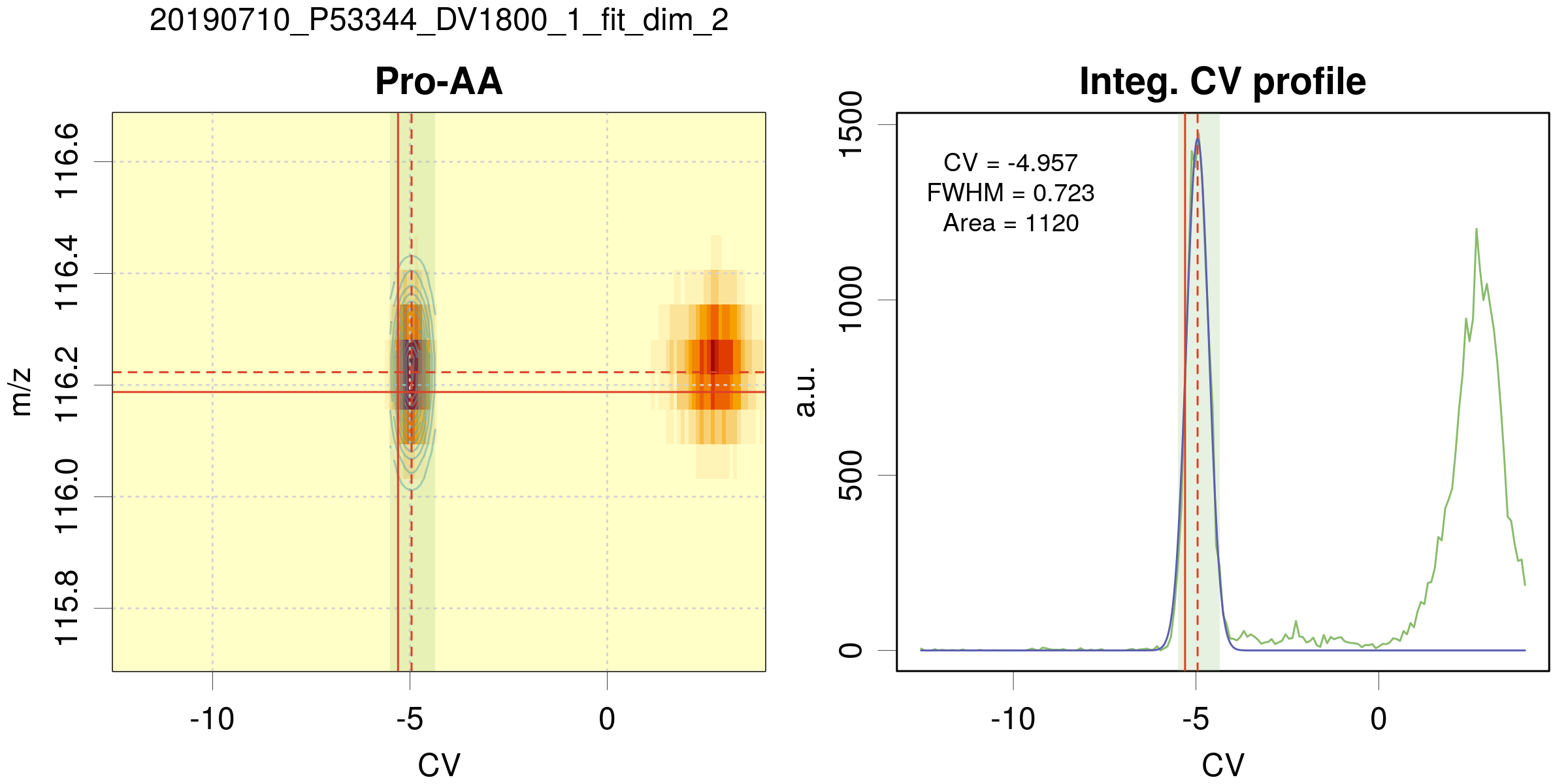
-
On the left panel, the 2D map centered on the peak position. The data are coded in color intensity from pale yellow to red. The pale blue-green area is the CV search range for the peak position. The solid red lines depict the peak position defined by
m/z_refandCV_refin the targets table. The dashed red lines correspond to the estimated peak position. If the 2D fit is successful, green contour lines of the peak are displayed. -
On the right panel, the CV peak profile for data integrated over m/z (green curve). The blue line is the best fit. The red lines and pale blue have the same meaning as above. The best-fit parameters are reported in the graph, with a warning in case of fit problems.
Example of a 1D fit along m/z (fit_dim=0) 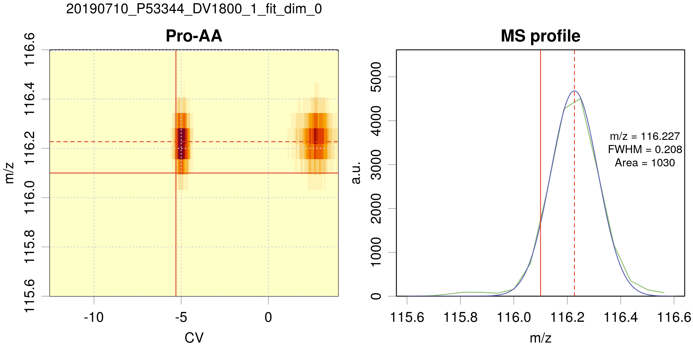
- Same legend as for the 2D fit, except for the right panel, which represents the m/z profile of the peak.
Tables
For each experiments/task associated with (MS_file, DMS_file), three
comma delimited ‘.csv’ files are generated: prefix_results.csv,
prefix_fit.csv and prefix_XIC.csv.
For each task, a file names prefix_ctrlParams.yaml is also generated
for reproducibility purpose. It contains the values of all the control
variables for this task.
Notes
- In output files, the missing data are represented by
NAs.
Fit results: XXX_results.csv
-
the first 4 columns are copies of the
tgTabledata:Name Comments m/z_ref CV_ref -
the next 8 columns correspond to the position, width and uncertainty values of the optimized Gaussian in the m/z and CV dimensions (unavailable data are represented by
NA)m/z u_m/z CV u_CV FWHM_m/z u_FWHM_m/z FWHM_CV u_FWHM_CV -
the next 2 columns are the results for the optimized Area values, and corresponding uncertainty.
Area u_Area -
finally, you will find the
fit_dimvalue, thediluindex, and thetagwhich is a concatenation of date + MS_filename + fit_dim that can be used for further sorting of the results.fit_dim dilu tag
Peak profiles: XXX_fit.csv and XXX_XIC.csv
The XXX_XIC.csv file contains the time/CV data profiles integrated
over m/z for the compounds in tgTable (fit_dim=1,2) or the m/z
data profile (fit_dim=0) for the species in tgTable. The
XXX_fit.csv file contains the corresponding gaussian peak profiles.
-
For
fit_dim=1,2, the first two columns are the time and CV abscissae of the profilestime CV For
fit_dim=0, the first column is m/zm/z -
the following columns are headed by the name of the compound and contain the corresponding profiles